Home
The running example
The underlying data is generated by: sin(2πx) + noise(Gauss‐
ian)
Probability theory provides a framework for expressing uncer‐
tainty in a precise and quantitative manner.
Decision theory allows us to exploit this probabilistic represen‐
tation in order to make predictions that are optimal according to
appropriate criteria.
Polynomial fitting:
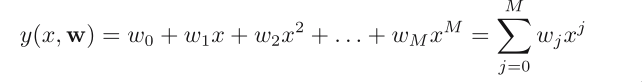 It is linear in the unknown parameters. Such models are called
linear models.
Now, how do we train and find the values of the unknown parame‐
ters?
The values of the coefficients will be determined by fitting the
polynomial to the training data.
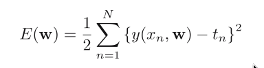
This can be done by minimizing an error function that measures
the misfit between the function and the training set data points.
One simple choice of error function is the sum of the squares of
the errors between the predictions for each data point and the
corresponding target values.
Minmize the error function:
It is linear in the unknown parameters. Such models are called
linear models.
Now, how do we train and find the values of the unknown parame‐
ters?
The values of the coefficients will be determined by fitting the
polynomial to the training data.
This can be done by minimizing an error function that measures
the misfit between the function and the training set data points.
One simple choice of error function is the sum of the squares of
the errors between the predictions for each data point and the
corresponding target values.
Minmize the error function:
 We can solve the curve fitting problem by choosing the value of w
for which E(w) is as small as possible.
There remains the problem of choosing the order M of the polyno‐
mial.
By choosing a large order M, we trained an over‐fitting model.
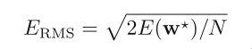
RMS: root mean square
We can solve the curve fitting problem by choosing the value of w
for which E(w) is as small as possible.
There remains the problem of choosing the order M of the polyno‐
mial.
By choosing a large order M, we trained an over‐fitting model.
RMS: root mean square
 ‐2‐
The division by N allows us to compare different sizes of data
sets on an equal footing, and the square root ensures that E_RMS
is measured on the same scale (and in the same units) as the tar‐
get variable t.
We might suppose that the best predictor for new data would be
the function sin(2πx) from which the data was generated (and this
is indeed the case)
A power series expansion of the function sin(2πx) contains terms
of all orders, so we might expect that results should improve mo‐
notonically as we increase M.
However, by increasing M, we get over‐fitting, which is counter
intuitive.
We can gain some insight into the problem by examine the vlaues
of the coefficients w* obtained from polynomials of various or‐
der.
As M increases, the magnitude of the coefficients typically gets
larger.
‐2‐
The division by N allows us to compare different sizes of data
sets on an equal footing, and the square root ensures that E_RMS
is measured on the same scale (and in the same units) as the tar‐
get variable t.
We might suppose that the best predictor for new data would be
the function sin(2πx) from which the data was generated (and this
is indeed the case)
A power series expansion of the function sin(2πx) contains terms
of all orders, so we might expect that results should improve mo‐
notonically as we increase M.
However, by increasing M, we get over‐fitting, which is counter
intuitive.
We can gain some insight into the problem by examine the vlaues
of the coefficients w* obtained from polynomials of various or‐
der.
As M increases, the magnitude of the coefficients typically gets
larger.
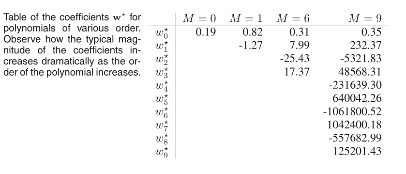 What is happening is that the more flexible polynomials with
larger values of M are becoming increasingly tuned to the random
noise on the target values.
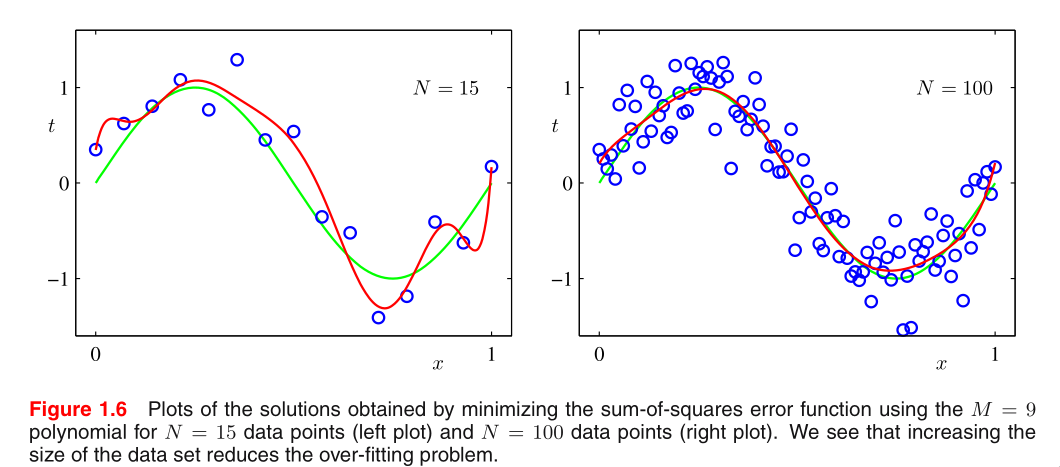
For a given model complexity, the over‐fitting problem become
less severe as the size of the data set increases.
What is happening is that the more flexible polynomials with
larger values of M are becoming increasingly tuned to the random
noise on the target values.
For a given model complexity, the over‐fitting problem become
less severe as the size of the data set increases.
 But why is least squares a good choice for an error function?
We shall see that the least squares approach to finding the model
parameters represents a specific case of maximum likelihood, and
that the over‐fitting problem can be understood as a general
property of maximum likelihood.
By adopting a Bayesian approach, the over‐fitting problem can be
avoided.
We shall see that there is no difficulty from a Bayesian perspec‐
tive in employing models for which the number of parameters
greatly exceeds the number of data points. Indeed, in a Bayesian
model the effective number of parameters adapts automatically to
the size of the data set.
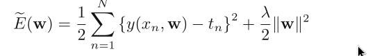
One technique that is often used to control the over‐fitting phe‐
nomenon in such cases is that of regularization, which involves
‐3‐
adding a penalty term to the error function in order to discour‐
age the coefficients from reaching large values.
But why is least squares a good choice for an error function?
We shall see that the least squares approach to finding the model
parameters represents a specific case of maximum likelihood, and
that the over‐fitting problem can be understood as a general
property of maximum likelihood.
By adopting a Bayesian approach, the over‐fitting problem can be
avoided.
We shall see that there is no difficulty from a Bayesian perspec‐
tive in employing models for which the number of parameters
greatly exceeds the number of data points. Indeed, in a Bayesian
model the effective number of parameters adapts automatically to
the size of the data set.
One technique that is often used to control the over‐fitting phe‐
nomenon in such cases is that of regularization, which involves
‐3‐
adding a penalty term to the error function in order to discour‐
age the coefficients from reaching large values.
 Different penalties:
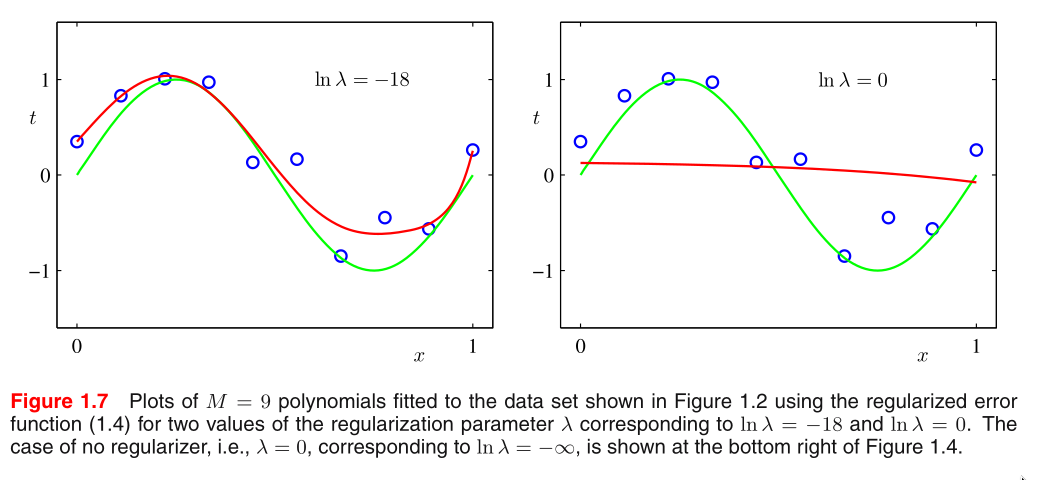 Large penalties turn the prediction curves into smooth ones.
Note that often the coefficient w_0 is omitted from the regular‐
izer because its inclusion causes the results to depend on the
choice of origin for the target variable.
The particular case of a quadratic regularizer is called ridge
regression. In the context of neural networks, this approach is
known as weight decay.
Large penalties turn the prediction curves into smooth ones.
Note that often the coefficient w_0 is omitted from the regular‐
izer because its inclusion causes the results to depend on the
choice of origin for the target variable.
The particular case of a quadratic regularizer is called ridge
regression. In the context of neural networks, this approach is
known as weight decay.
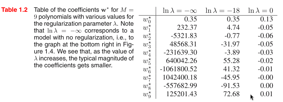 The regularization has the desired effect of reducing the magni‐
tude of the coefficients.
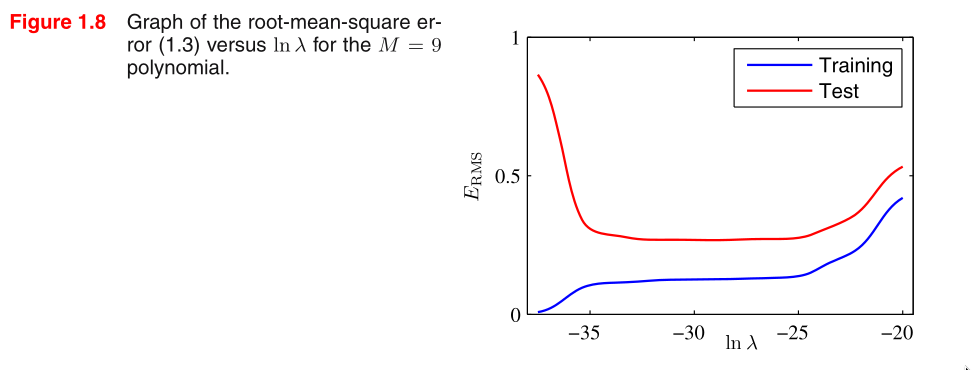
The impact of the regularization term on the generalization error
can be seen by plotting the value of the RMS error for both
training and test sets against ln λ
We see that in effect λ now controls the effective complexity of
the model and hence determines the degree of over‐fitting.
The regularization has the desired effect of reducing the magni‐
tude of the coefficients.
The impact of the regularization term on the generalization error
can be seen by plotting the value of the RMS error for both
training and test sets against ln λ
We see that in effect λ now controls the effective complexity of
the model and hence determines the degree of over‐fitting.
 The issue of model complexity is an important one.
How do we optimize the model complexity (either M or λ )?
Partitioning it into a training set, used to determine the coef‐
ficients w, and a separate validation set, also called a hold‐out
set, used to optimize the model complexity. In many cases, how‐
ever, this will prove to be too wasteful of valuable training
data.
But why is least squares a good choice for an error function?
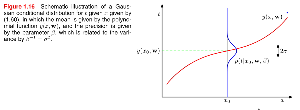
With probability theory, we can express our uncertainty over
the value of the target variable using a probability distribu‐
tion.
‐4‐
We shall assume that, given the value of x, the corresponding
value of t has a Gaussian distribution with a mean equal to the
value y(x, w) of the polynomial curve.
The issue of model complexity is an important one.
How do we optimize the model complexity (either M or λ )?
Partitioning it into a training set, used to determine the coef‐
ficients w, and a separate validation set, also called a hold‐out
set, used to optimize the model complexity. In many cases, how‐
ever, this will prove to be too wasteful of valuable training
data.
But why is least squares a good choice for an error function?
With probability theory, we can express our uncertainty over
the value of the target variable using a probability distribu‐
tion.
‐4‐
We shall assume that, given the value of x, the corresponding
value of t has a Gaussian distribution with a mean equal to the
value y(x, w) of the polynomial curve.
 Conclusion: the sum‐of‐squares error function has arisen as a
consequence of maximizing likelihood under the assumption of a
Gaussian noise distribution.
What is Bayesian approach?
Conclusion: the sum‐of‐squares error function has arisen as a
consequence of maximizing likelihood under the assumption of a
Gaussian noise distribution.
What is Bayesian approach?