Home
SVM
Support Vector Machines
It is a theoretically well motivated and practically effec‐
tive classification algorithm.
It is also called maximum margin classifier.
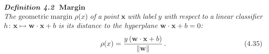
The theoretical foundation for SVMs is the notion of margin.
separable datasets
There are infinitely many such separating hyperplanes. Which
hyperplane should a learning algorithm select?
SVM chooses the hyperplane with the maximum margin. Known as the
maximum‐margin hyperplane.
The SVM solution can be viewed as the "safest" choice in the fol‐
lowing sense: A test point is classified correctly by a separat‐
ing hyperplane with margin ρ even when it falls within a distance
ρ of the training samples sharing the same label. (Here training
samples mean sample points?)
For the SVM solution, ρ is the maximum margin and thus the
"safest" value.
Primal optimization problem
The general equation of a hyperplane
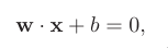 w is normal to the hyperplane.
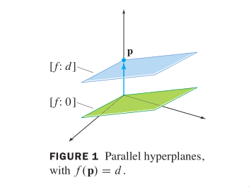 (The set of solutions of Ax=b is obtained by translating the so‐
lution set of Ax=0, using any particular solution p of Ax=b.)
When A is the standard matrix of the transformation f, this says
that
‐2‐
[f:d]=[f:0]+p for any p in [f:d]
When A is a 1 x n matrix, the equation Ax=d may be written with
an inner product <n,x>. Then [f:0] = {x: <n,x>=0}, which shows
that [f:0] is the orthogonal complement of the subspace spanned
by n. In the terminology of calculus and geometry, n is called a
normal vector to [f:0]. (A "normal" vector in this sense need not
have unit length.) Also, n is said to be normal to each parallel
hyperplane [f:d], even though <n,x> is not zero when d != 0.
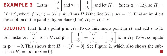
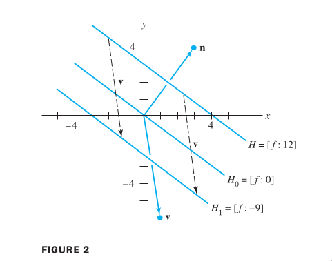
Example hyperplanes:
(The set of solutions of Ax=b is obtained by translating the so‐
lution set of Ax=0, using any particular solution p of Ax=b.)
When A is the standard matrix of the transformation f, this says
that
‐2‐
[f:d]=[f:0]+p for any p in [f:d]
When A is a 1 x n matrix, the equation Ax=d may be written with
an inner product <n,x>. Then [f:0] = {x: <n,x>=0}, which shows
that [f:0] is the orthogonal complement of the subspace spanned
by n. In the terminology of calculus and geometry, n is called a
normal vector to [f:0]. (A "normal" vector in this sense need not
have unit length.) Also, n is said to be normal to each parallel
hyperplane [f:d], even though <n,x> is not zero when d != 0.
Example hyperplanes:
 Note that this definition of a hyperplane is invariant to non‐
zero scalar multiplication.
Hence, for a hyperplane that does not pass through any sample
point, we can scale w and b appropriately such that min |<w,x> +
b| = 1. (w is normal to the hyperplane, but here we scale the
norm to 1. This has nothing to do with the concept of normal.
This is the marginal hyperplane.)
Note that this definition of a hyperplane is invariant to non‐
zero scalar multiplication.
Hence, for a hyperplane that does not pass through any sample
point, we can scale w and b appropriately such that min |<w,x> +
b| = 1. (w is normal to the hyperplane, but here we scale the
norm to 1. This has nothing to do with the concept of normal.
This is the marginal hyperplane.)
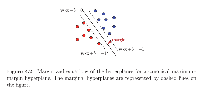 min |<w,x> + b| = 1, these x(s) are the support vectors. Support
vectors determine the marginal hyperplanes.
min |<w,x> + b| = 1, these x(s) are the support vectors. Support
vectors determine the marginal hyperplanes.
 The logic sequence:
1. We decided to use <w,x> + b = 0 as the classifier. First, we
choose a w, and it determines the angle of the hyperplane. Then
by choosing b we make the hyperplane lies in the middle, so that
the closest points on both sides are at the same distance. Be‐
cause this sounds natural to do.
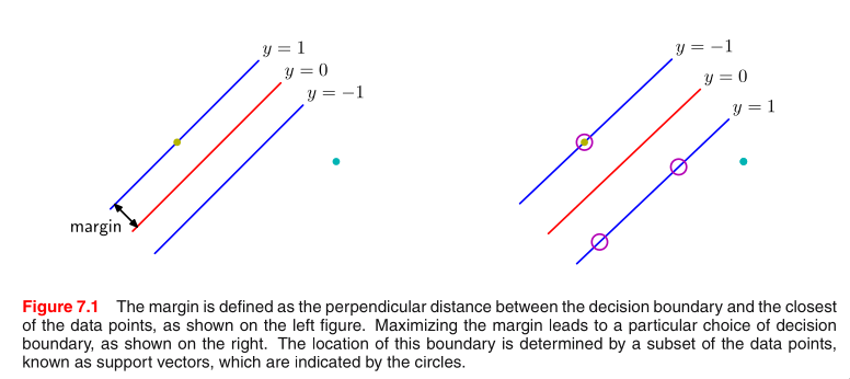
2. On both sides of the hyperplane, there are training points
that are closest to the hyperplane <w,x> + b = 0. These are the
support vectors.
3. Support vectors determine two hyperplanes: <w, x_1> + b = c,
<w, x_2> + b = ‐c. These two hyperplanes are invariant to multi‐
plication, therefore, we can scale it to <w/c, x_1> + b/c = 1. In
this way, we simplify the problem and save ourselves from the
trouble of dealing with c. Optimizing over (w,b) is no different
to optimizing over (w/c,b/c). And we will treat (w/c,b/c) as the
new (w,b) we want to optimize on.
4. Now we have 3 hyperplanes. Our goal is to optimize w and b
‐3‐
according to some criteria. Therefore we need to know the dis‐
tance. The criteria is to choose the one that maximizes the dis‐
tance, that is, the margin.
5. We measure the margin in the direction of the normal vector,
that is, w. The margin is the distance between the separating hy‐
perplane and its marginal hyperplane.
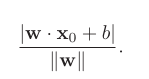
6. x_0 is not on the hyperplane <w, x> + b = 0. We add cw to x_0,
so that x_1 = x_0 + cw is on the hyperplane. Here c is a con‐
stant. Then <w, x_1> + b = 0. <w, x_0 + cw> + b = 0. The distance
is ||cw||. We solve the equation and found that ||cw|| = |<w,x_0>
+ b| / ||w||
The distance of any point to a hyperplane:
The logic sequence:
1. We decided to use <w,x> + b = 0 as the classifier. First, we
choose a w, and it determines the angle of the hyperplane. Then
by choosing b we make the hyperplane lies in the middle, so that
the closest points on both sides are at the same distance. Be‐
cause this sounds natural to do.
2. On both sides of the hyperplane, there are training points
that are closest to the hyperplane <w,x> + b = 0. These are the
support vectors.
3. Support vectors determine two hyperplanes: <w, x_1> + b = c,
<w, x_2> + b = ‐c. These two hyperplanes are invariant to multi‐
plication, therefore, we can scale it to <w/c, x_1> + b/c = 1. In
this way, we simplify the problem and save ourselves from the
trouble of dealing with c. Optimizing over (w,b) is no different
to optimizing over (w/c,b/c). And we will treat (w/c,b/c) as the
new (w,b) we want to optimize on.
4. Now we have 3 hyperplanes. Our goal is to optimize w and b
‐3‐
according to some criteria. Therefore we need to know the dis‐
tance. The criteria is to choose the one that maximizes the dis‐
tance, that is, the margin.
5. We measure the margin in the direction of the normal vector,
that is, w. The margin is the distance between the separating hy‐
perplane and its marginal hyperplane.
6. x_0 is not on the hyperplane <w, x> + b = 0. We add cw to x_0,
so that x_1 = x_0 + cw is on the hyperplane. Here c is a con‐
stant. Then <w, x_1> + b = 0. <w, x_0 + cw> + b = 0. The distance
is ||cw||. We solve the equation and found that ||cw|| = |<w,x_0>
+ b| / ||w||
The distance of any point to a hyperplane:
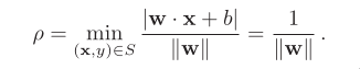
 For canonical hyperplane, the margin ρ is given by
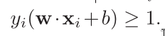
 So far, we’ve only discussed about margins. To classify cor‐
rectly, there is one constraint to keep.
So far, we’ve only discussed about margins. To classify cor‐
rectly, there is one constraint to keep.
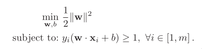
 Finally, we have transformed the original problem into a convex
optimization problem. The original problem is: a hyperplane max‐
imizing the margin while correctly classifying all training
points.
Finally, we have transformed the original problem into a convex
optimization problem. The original problem is: a hyperplane max‐
imizing the margin while correctly classifying all training
points.
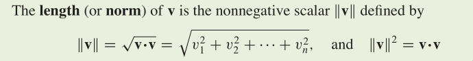
 What is the difference between | | and || || ?
| | is the absolute value. || || is the norm.
Dot product and norm:
What is the difference between | | and || || ?
| | is the absolute value. || || is the norm.
Dot product and norm:
 A canonical hyperplane is the one of separating hyperplane with
both its marginal hyperplane |<w,x> + b| = 1.
Therefore, maximizing the margin of a canonical hyperplane is
equivalent to minimizing ||w||. In optimization problem, we usu‐
ally minimize (1/2)||w||ˆ2.
‐4‐
The objective function F: w ‐> (1/2)||w||ˆ2 is infinitely differ‐
entiable. Its gradient is w. Its Hessian is the identity matrix
I, whose eigenvalues are strictly positive. Therefore F is
strictly convex.
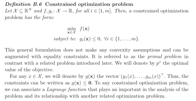
The constraints are all defined by affine functions and are thus
qualified.
Thus, in view of the results known for convex optimization, the
optimization problem admits a unique solution, an important and
favorable property that does not hold for all learning algo‐
rithms.
Constrained optimization problem:
A canonical hyperplane is the one of separating hyperplane with
both its marginal hyperplane |<w,x> + b| = 1.
Therefore, maximizing the margin of a canonical hyperplane is
equivalent to minimizing ||w||. In optimization problem, we usu‐
ally minimize (1/2)||w||ˆ2.
‐4‐
The objective function F: w ‐> (1/2)||w||ˆ2 is infinitely differ‐
entiable. Its gradient is w. Its Hessian is the identity matrix
I, whose eigenvalues are strictly positive. Therefore F is
strictly convex.
The constraints are all defined by affine functions and are thus
qualified.
Thus, in view of the results known for convex optimization, the
optimization problem admits a unique solution, an important and
favorable property that does not hold for all learning algo‐
rithms.
Constrained optimization problem:
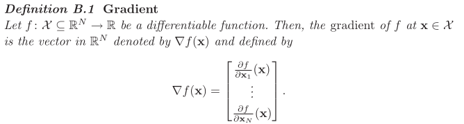
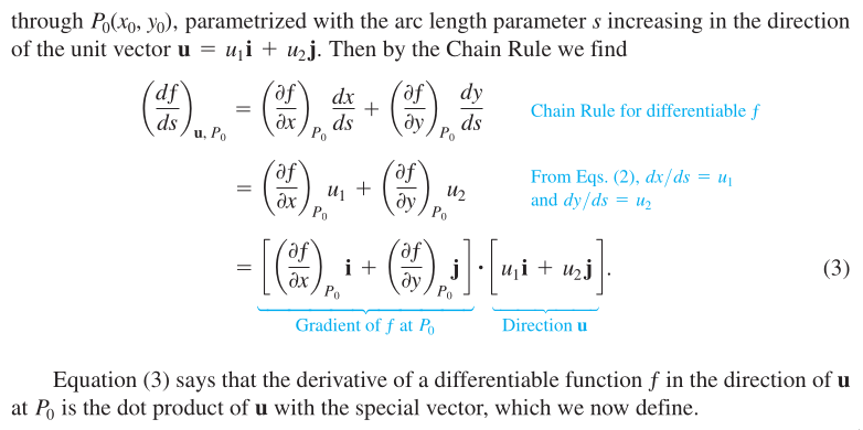
 Gradient vectors:
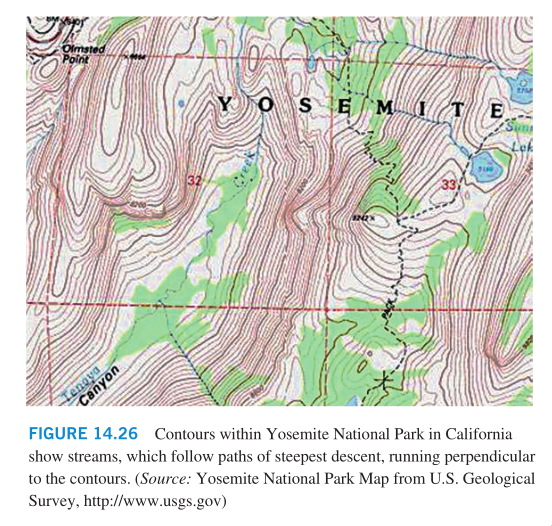
 If you look at the map showing contours within Yosemite National
Park in California, you will notice that the streams flow perpen‐
dicular to the contours. The streams are following paths of
steepest descent so the waters reach lower elevations as quickly
as possible. Therefore, the fastest instantaneous rate of change
in a stream’s elevation above sea level has a particular direc‐
tion.
If you look at the map showing contours within Yosemite National
Park in California, you will notice that the streams flow perpen‐
dicular to the contours. The streams are following paths of
steepest descent so the waters reach lower elevations as quickly
as possible. Therefore, the fastest instantaneous rate of change
in a stream’s elevation above sea level has a particular direc‐
tion.
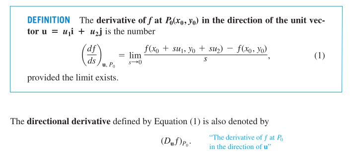
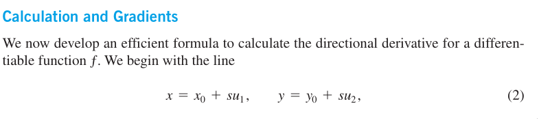
 Directional derivative:
 An example of computing directional derivative:
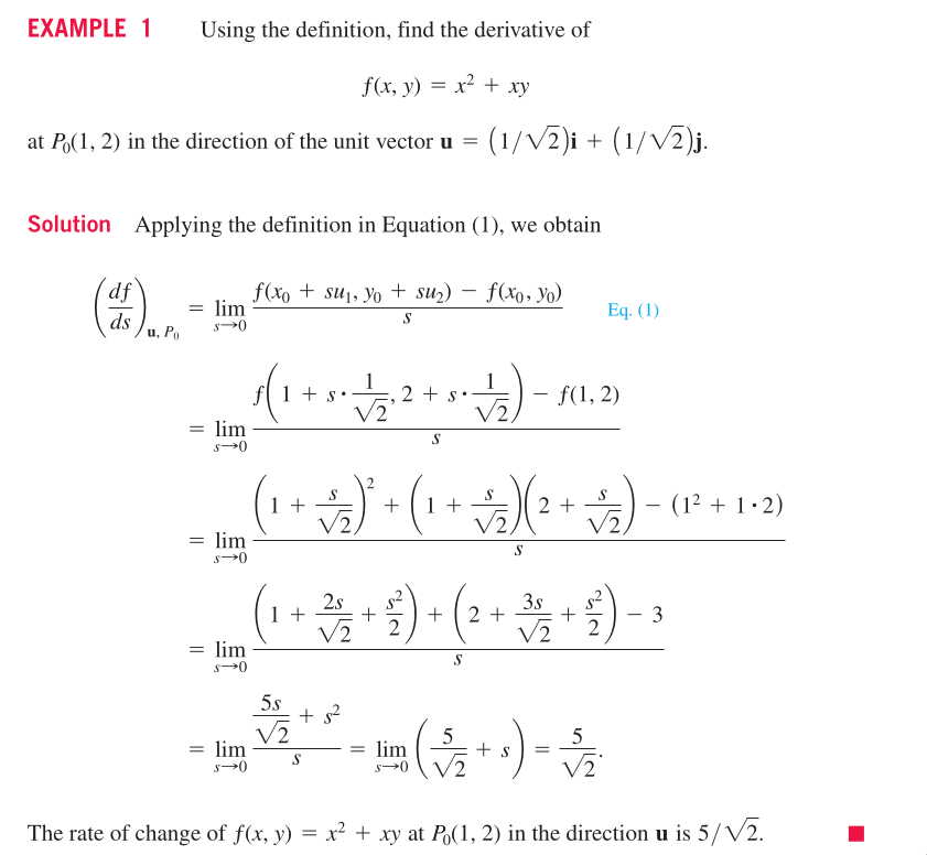 This means by moving (x,y) one unit in the direction of u, the
value of f increases 5/sqrt(2)
Why do we need directional derivative?
When we study derivative, we try to understand the relationship
between the value of a function and its variables, that is, how
do they change with respect to each other? The nature of a deriv‐
ative is a limitation.
But how does directional derivative related to partial deriva‐
tive?
‐5‐
The nature of a partial derivative is still a limitation. But
this time, only one variable moves, and all others are fixed. In
the case of directional derivative, x is moving in all direc‐
tions. We put them together so that we can see the difference
clearly.
This means by moving (x,y) one unit in the direction of u, the
value of f increases 5/sqrt(2)
Why do we need directional derivative?
When we study derivative, we try to understand the relationship
between the value of a function and its variables, that is, how
do they change with respect to each other? The nature of a deriv‐
ative is a limitation.
But how does directional derivative related to partial deriva‐
tive?
‐5‐
The nature of a partial derivative is still a limitation. But
this time, only one variable moves, and all others are fixed. In
the case of directional derivative, x is moving in all direc‐
tions. We put them together so that we can see the difference
clearly.
 Here we see that when we talk about directional derivative, we
need to specify a unit vector and the changing rate is about
changing in all directions at the same time. However, when we
talk about partial derivative, we talk about the changing in only
one direction. It looks like there is some connection between the
two.
Now we are interested in the gradients and Hessians, which of
these derivatives do we need?
From the example above, it is so much work to compute a direc‐
tional derivative, are there any better ways to go? That is how
the gradient comes to help.
Here we see that when we talk about directional derivative, we
need to specify a unit vector and the changing rate is about
changing in all directions at the same time. However, when we
talk about partial derivative, we talk about the changing in only
one direction. It looks like there is some connection between the
two.
Now we are interested in the gradients and Hessians, which of
these derivatives do we need?
From the example above, it is so much work to compute a direc‐
tional derivative, are there any better ways to go? That is how
the gradient comes to help.
 This makes sense since the directional derivative is the combina‐
tional effects of all the partial derivatives effecting at the
same time. That is how the concepts of partial derivatives, di‐
rectional derivative and gradient relate.
This makes sense since the directional derivative is the combina‐
tional effects of all the partial derivatives effecting at the
same time. That is how the concepts of partial derivatives, di‐
rectional derivative and gradient relate.
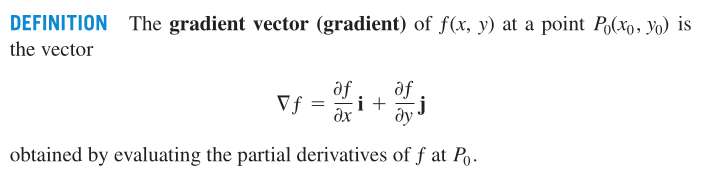 The gradient has nothing to do with the unit vector. The unit
vector gains a role when directional derivative is computed.
Therefore, the directional derivative is a dot product.
We study directional derivative because we want to find out ex‐
trem values and saddle points of a function.
Continuous functions of two variables assume extreme values on
closed, bounded domains.
The gradient has nothing to do with the unit vector. The unit
vector gains a role when directional derivative is computed.
Therefore, the directional derivative is a dot product.
We study directional derivative because we want to find out ex‐
trem values and saddle points of a function.
Continuous functions of two variables assume extreme values on
closed, bounded domains.
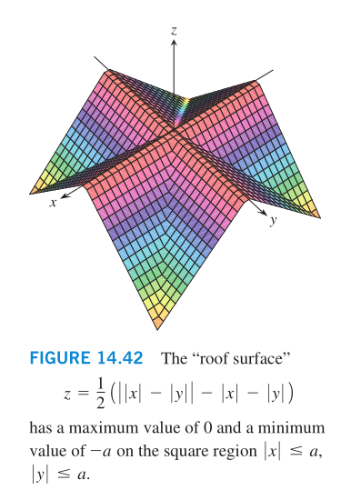
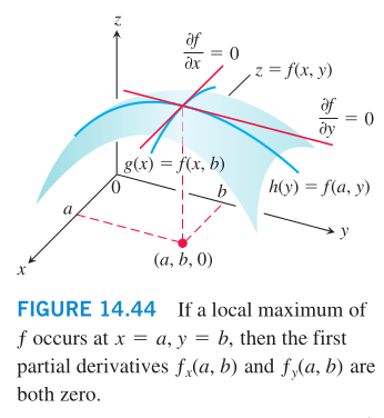
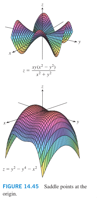
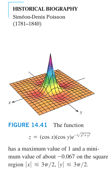 A function of two variables can assume extreme values only at do‐
main boundary points or at interior domain points where both
first partial derivatives are zero or where one or both of the
first partial derivatives fail to exist. These only ensures local
maxima or local minima. However, the vanishing of derivatives at
an interior point (a,b) does not always signal the presence of an
‐6‐
extreme value. The surface that is the graph of the function
might be shaped like a saddle right above (a,b) and cross its
tangent plane there.
A function of two variables can assume extreme values only at do‐
main boundary points or at interior domain points where both
first partial derivatives are zero or where one or both of the
first partial derivatives fail to exist. These only ensures local
maxima or local minima. However, the vanishing of derivatives at
an interior point (a,b) does not always signal the presence of an
‐6‐
extreme value. The surface that is the graph of the function
might be shaped like a saddle right above (a,b) and cross its
tangent plane there.
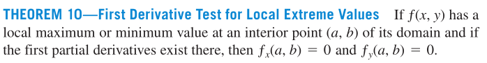
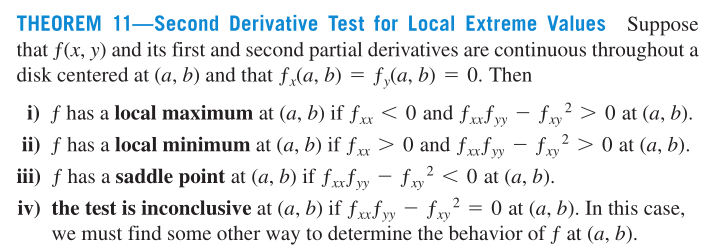
 As with functions of a single variable, the key to identifying
the local extrema is the First Derivative Test.
As with functions of a single variable, the key to identifying
the local extrema is the First Derivative Test.
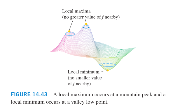 To find the local extreme values of a function of a single vari‐
able, we look for points where the graph has a horizontal tangent
line. At such points, we then look for local maxima, local min‐
ima, and points of inflection. For a function f(x,y) of two vari‐
ables, we look for points where the surface z=f(x,y) has a hori‐
zontal tangent plane. At such points, we then look for local max‐
ima, local minima, and saddle points.
Local extrema are also called relative extrema.
First Derivative Test:
To find the local extreme values of a function of a single vari‐
able, we look for points where the graph has a horizontal tangent
line. At such points, we then look for local maxima, local min‐
ima, and points of inflection. For a function f(x,y) of two vari‐
ables, we look for points where the surface z=f(x,y) has a hori‐
zontal tangent plane. At such points, we then look for local max‐
ima, local minima, and saddle points.
Local extrema are also called relative extrema.
First Derivative Test:
 To solve a convex optimization, we take the gradient of the func‐
tion and set it to 0. Then why do we need to know about Hessian?
To solve a convex optimization, we take the gradient of the func‐
tion and set it to 0. Then why do we need to know about Hessian?
 First and second derivative tests (for finding extreme values)
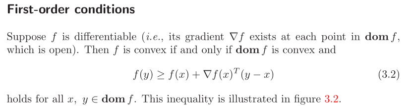
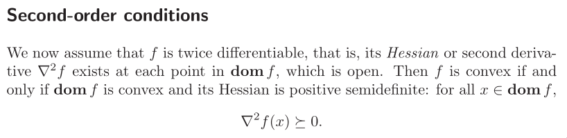
 First and second order conditions (for determining convexity)
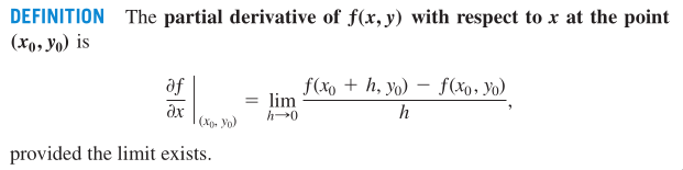
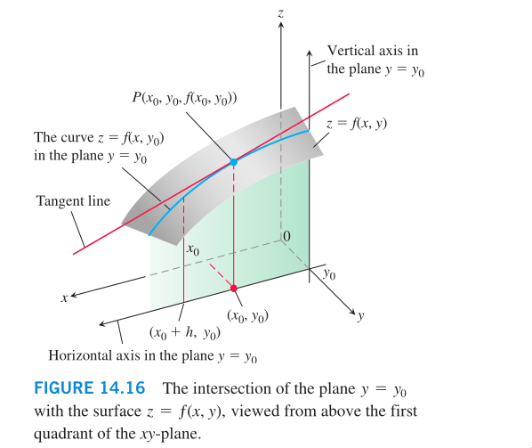
 Partial derivative:
The calculus of several variables is similar to single‐variable
‐7‐
calculus applied to several variables one at a time. When we hold
all but one of the independent variables of a function constant
and differentiate with respect to that one variable, we get a
"partial" derivative.
An equivalent expression for the partial derivative is
Partial derivative:
The calculus of several variables is similar to single‐variable
‐7‐
calculus applied to several variables one at a time. When we hold
all but one of the independent variables of a function constant
and differentiate with respect to that one variable, we get a
"partial" derivative.
An equivalent expression for the partial derivative is
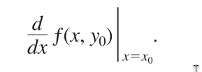 To distinguish partial derivatives from ordinary derivatives we
use the symbol
To distinguish partial derivatives from ordinary derivatives we
use the symbol
 rather than the d previously used.
Partial derivative geometrically:
rather than the d previously used.
Partial derivative geometrically:
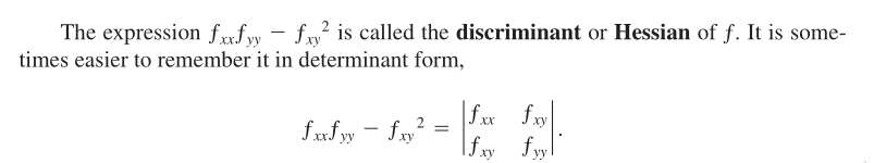
 Hessian matrix:
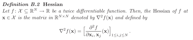 Hessian is also called second derivative.
Why is Hessian important? Answer: Second‐order conditions. With
these conditions, we determine f’s convexity.
For a function on R, this reduces to the simple condition f’’(x)
>= 0, which means that the derivative is nondecreasing.
Question: if we already know the gradient vector, can we compute
Hessian matrix from that?
Second derivative means taking derivative at a time and then an‐
other time, these 2 times don’t happen at the same time. There‐
fore the first time of taking the derivate of ||w||ˆ2 already
filters out all other terms unrelated to w_i. Hence, the final
result is the identity matrix I, rather than things like w_i +
w_j (this only happens when we treat w_i and w_j as independent
variables and all others as constant, which doesn’t make sense.
By definition of derivative, the operation only works on one
variable at a time).
‐8‐
How do we compute gradient for the square of norm?
Taking partial derivatives for each direction in w, the gradient
vector is the vector of partial derivatives, that is, w itself
(Here we see the reason why we have put the factor 1/2 in the op‐
timization problem).
Hyperplanes will be important for understanding the multidimen‐
sional nature of the linear programming problems.
Dual optimization problem
non‐separable datasets
the problem of linear classification
Input space X
Output/Target space Y = {‐1, +1}
Target function f: X‐>Y
Given a hypothesis set H of functions mapping X to Y
Training sample S of size m drawn i.i.d. from X (unknown distrib‐
ution D)
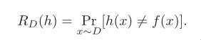
The problem consists of determining a hypothesis h from H, a bi‐
nary classifier, with small generalization error.
Hessian is also called second derivative.
Why is Hessian important? Answer: Second‐order conditions. With
these conditions, we determine f’s convexity.
For a function on R, this reduces to the simple condition f’’(x)
>= 0, which means that the derivative is nondecreasing.
Question: if we already know the gradient vector, can we compute
Hessian matrix from that?
Second derivative means taking derivative at a time and then an‐
other time, these 2 times don’t happen at the same time. There‐
fore the first time of taking the derivate of ||w||ˆ2 already
filters out all other terms unrelated to w_i. Hence, the final
result is the identity matrix I, rather than things like w_i +
w_j (this only happens when we treat w_i and w_j as independent
variables and all others as constant, which doesn’t make sense.
By definition of derivative, the operation only works on one
variable at a time).
‐8‐
How do we compute gradient for the square of norm?
Taking partial derivatives for each direction in w, the gradient
vector is the vector of partial derivatives, that is, w itself
(Here we see the reason why we have put the factor 1/2 in the op‐
timization problem).
Hyperplanes will be important for understanding the multidimen‐
sional nature of the linear programming problems.
Dual optimization problem
non‐separable datasets
the problem of linear classification
Input space X
Output/Target space Y = {‐1, +1}
Target function f: X‐>Y
Given a hypothesis set H of functions mapping X to Y
Training sample S of size m drawn i.i.d. from X (unknown distrib‐
ution D)
The problem consists of determining a hypothesis h from H, a bi‐
nary classifier, with small generalization error.
 Question: How do we choose H? Answer: follow Occam’s razor prin‐
ciple.
‐9‐
Margin theory
What do we want? generalization bounds.
Question: How do we choose H? Answer: follow Occam’s razor prin‐
ciple.
‐9‐
Margin theory
What do we want? generalization bounds.
 Occam’s razor principle
Hyperthesis sets with smaller complexity ‐‐ e.g., smaller
VC‐dimension or Rademacher complexity ‐‐ provide better learning
guarantees.
A natural hypothesis set with relatively small complexity is that
of linear classifiers
Occam’s razor principle
Hyperthesis sets with smaller complexity ‐‐ e.g., smaller
VC‐dimension or Rademacher complexity ‐‐ provide better learning
guarantees.
A natural hypothesis set with relatively small complexity is that
of linear classifiers
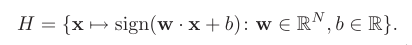 A hypothesis of the form x ‐> sign(<w,x> + b) thus labels posi‐
tively all points falling on one side of the hyperplane <w,x> + b
= 0 and negatively all others.
The problem is referred to as a linear classification problem.
Hyperplane
Check geometry_of_vector_spaces.m
A hypothesis of the form x ‐> sign(<w,x> + b) thus labels posi‐
tively all points falling on one side of the hyperplane <w,x> + b
= 0 and negatively all others.
The problem is referred to as a linear classification problem.
Hyperplane
Check geometry_of_vector_spaces.m